What is the Jupyter Notebook?
Introduction
The Jupyter Notebook is an interactive computing environment that enables users to author notebook documents that include: - Live code - Interactive widgets - Plots - Narrative text - Equations - Images - Video
These documents provide a complete and self-contained record of a computation that can be converted to various formats and shared with others using email, Dropbox, version control systems (like git/GitHub) or nbviewer.jupyter.org.
Components
The Jupyter Notebook combines three components:
The notebook web application: An interactive web application for writing and running code interactively and authoring notebook documents.
Kernels: Separate processes started by the notebook web application that runs users’ code in a given language and returns output back to the notebook web application. The kernel also handles things like computations for interactive widgets, tab completion and introspection.
Notebook documents: Self-contained documents that contain a representation of all content visible in the notebook web application, including inputs and outputs of the computations, narrative text, equations, images, and rich media representations of objects. Each notebook document has its own kernel.
Notebook web application
The notebook web application enables users to:
Edit code in the browser, with automatic syntax highlighting, indentation, and tab completion/introspection.
Run code from the browser, with the results of computations attached to the code which generated them.
See the results of computations with rich media representations, such as HTML, LaTeX, PNG, SVG, PDF, etc.
Create and use interactive JavaScript widgets, which bind interactive user interface controls and visualizations to reactive kernel side computations.
Author narrative text using the Markdown markup language.
Include mathematical equations using LaTeX syntax in Markdown, which are rendered in-browser by MathJax.
Kernels
Through Jupyter’s kernel and messaging architecture, the Notebook allows code to be run in a range of different programming languages. For each notebook document that a user opens, the web application starts a kernel that runs the code for that notebook. Each kernel is capable of running code in a single programming language and there are kernels available in the following languages:
Python(ipython/ipython)
Julia (JuliaLang/IJulia.jl)
Ruby (minrk/iruby)
Haskell (gibiansky/IHaskell)
Scala (Bridgewater/scala-notebook)
node.js (https://gist.github.com/Carreau/4279371)
Go (takluyver/igo)
The default kernel runs Python code. The notebook provides a simple way for users to pick which of these kernels is used for a given notebook.
Each of these kernels communicate with the notebook web application and web browser using a JSON over ZeroMQ/WebSockets message protocol that is described here. Most users don’t need to know about these details, but it helps to understand that “kernels run code.”
Notebook documents
Notebook documents contain the inputs and outputs of an interactive session as well as narrative text that accompanies the code but is not meant for execution. Rich output generated by running code, including HTML, images, video, and plots, is embeddeed in the notebook, which makes it a complete and self-contained record of a computation.
When you run the notebook web application on your computer, notebook documents are just files on your local filesystem with a .ipynb extension. This allows you to use familiar workflows for organizing your notebooks into folders and sharing them with others.
Notebooks consist of a linear sequence of cells. There are three basic cell types:
Code cells: Input and output of live code that is run in the kernel
Markdown cells: Narrative text with embedded LaTeX equations
Raw cells: Unformatted text that is included, without modification, when notebooks are converted to different formats using nbconvert
Internally, notebook documents are JSON data with binary values base64 encoded. This allows them to be read and manipulated programmatically by any programming language. Because JSON is a text format, notebook documents are version control friendly.
Notebooks can be exported to different static formats including HTML, reStructeredText, LaTeX, PDF, and slide shows (reveal.js) using Jupyter’s nbconvert utility.
Furthermore, any notebook document available from a public URL or on GitHub can be shared via nbviewer. This service loads the notebook document from the URL and renders it as a static web page. The resulting web page may thus be shared with others without their needing to install the Jupyter Notebook.
------------------------------------------------------------------------------------------------
Notebook Basics
The Notebook dashboard
When you first start the notebook server, your browser will open to the notebook dashboard. The dashboard serves as a home page for the notebook. Its main purpose is to display the notebooks and files in the current directory. For example, here is a screenshot of the dashboard page for the examples directory in the Jupyter repository:
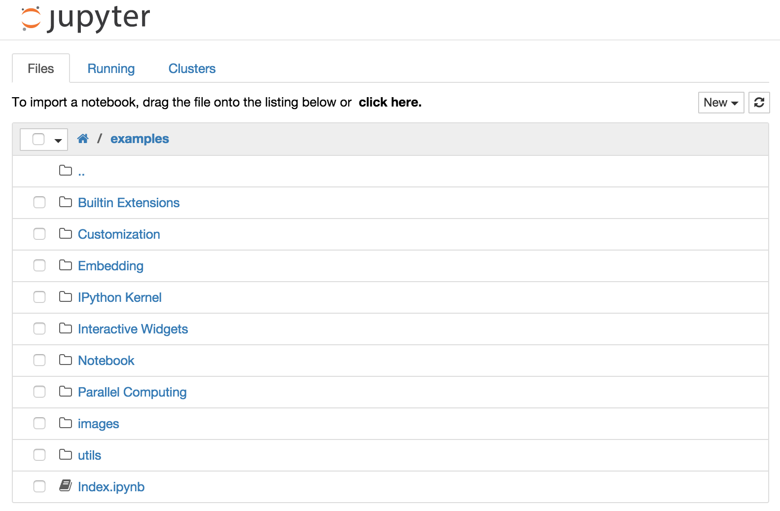
The top of the notebook list displays clickable breadcrumbs of the current directory. By clicking on these breadcrumbs or on sub-directories in the notebook list, you can navigate your file system.
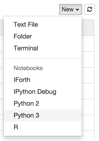
To create a new notebook, click on the “New” button at the top of the list and select a kernel from the dropdown (as seen below). Which kernels are listed depend on what’s installed on the server. Some of the kernels in the screenshot below may not exist as an option to you.
Notebooks and files can be uploaded to the current directory by dragging a notebook file onto the notebook list or by the “click here” text above the list.
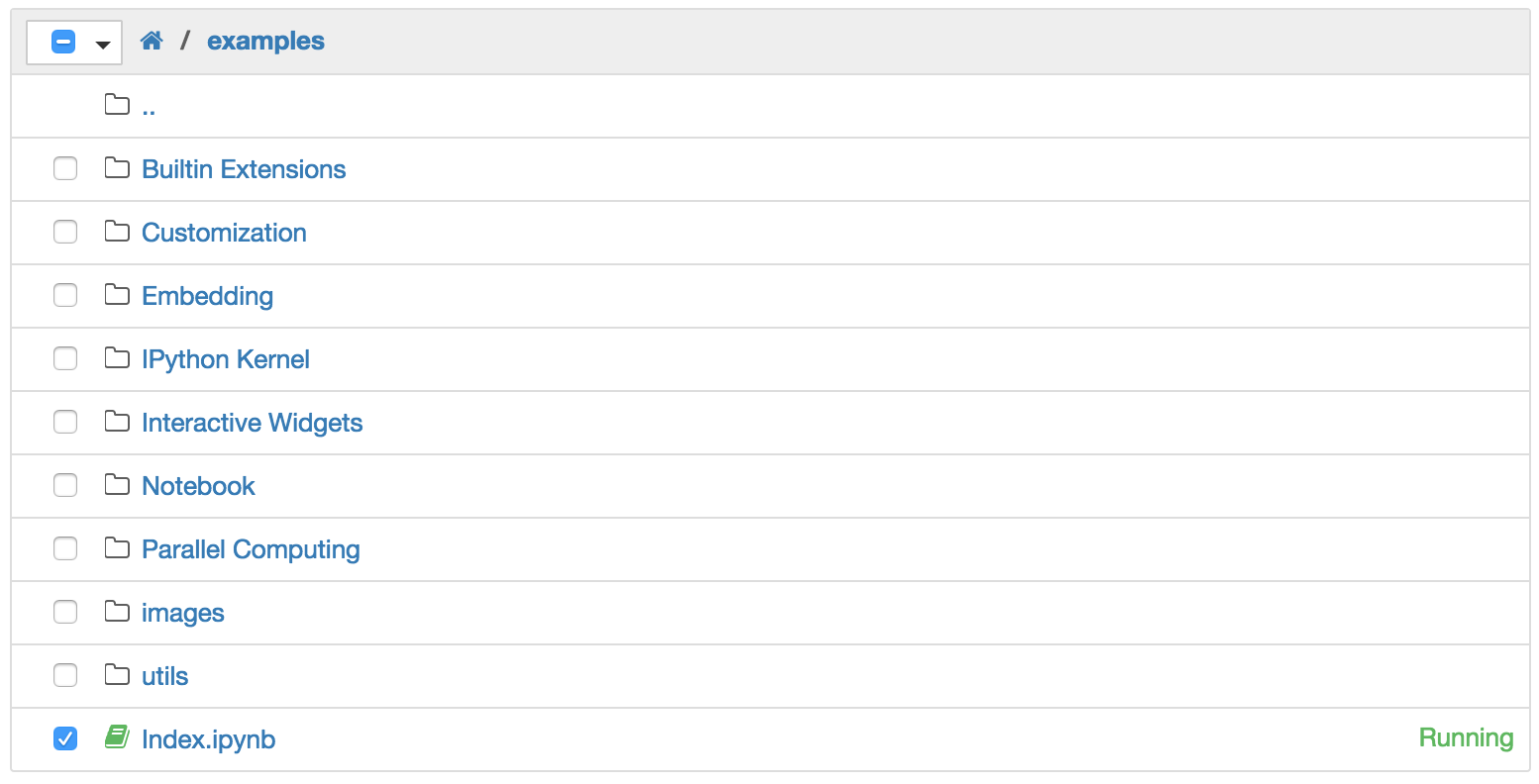
The notebook list shows green “Running” text and a green notebook icon next to running notebooks (as seen below). Notebooks remain running until you explicitly shut them down; closing the notebook’s page is not sufficient.
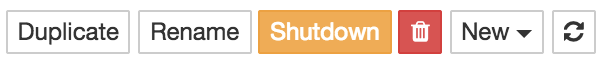
To shutdown, delete, duplicate, or rename a notebook check the checkbox next to it and an array of controls will appear at the top of the notebook list (as seen below). You can also use the same operations on directories and files when applicable.
To see all of your running notebooks along with their directories, click on the “Running” tab:
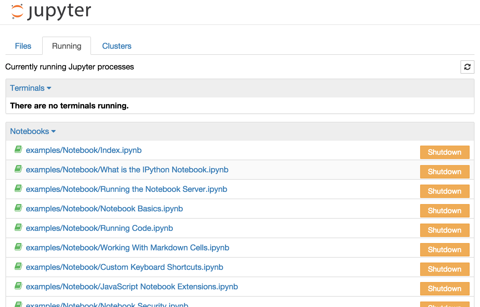
This view provides a convenient way to track notebooks that you start as you navigate the file system in a long running notebook server.
Overview of the Notebook UI
If you create a new notebook or open an existing one, you will be taken to the notebook user interface (UI). This UI allows you to run code and author notebook documents interactively. The notebook UI has the following main areas:
Menu
Toolbar
Notebook area and cells
The notebook has an interactive tour of these elements that can be started in the “Help:User Interface Tour” menu item.
Modal editor
Starting with IPython 2.0, the Jupyter Notebook has a modal user interface. This means that the keyboard does different things depending on which mode the Notebook is in. There are two modes: edit mode and command mode.
Edit mode
Edit mode is indicated by a green cell border and a prompt showing in the editor area:

When a cell is in edit mode, you can type into the cell, like a normal text editor.
Enter edit mode by pressing Enter or using the mouse to click on a cell’s editor area.
Command mode
Command mode is indicated by a grey cell border with a blue left margin:

When you are in command mode, you are able to edit the notebook as a whole, but not type into individual cells. Most importantly, in command mode, the keyboard is mapped to a set of shortcuts that let you perform notebook and cell actions efficiently. For example, if you are in command mode and you press c, you will copy the current cell - no modifier is needed.
Don’t try to type into a cell in command mode; unexpected things will happen!
Enter command mode by pressing Esc or using the mouse to click outside a cell’s editor area.
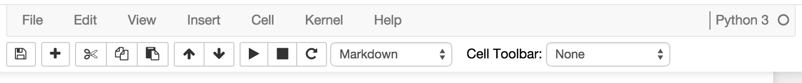
Mouse navigation
All navigation and actions in the Notebook are available using the mouse through the menubar and toolbar, which are both above the main Notebook area:
The first idea of mouse based navigation is that cells can be selected by clicking on them. The currently selected cell gets a grey or green border depending on whether the notebook is in edit or command mode. If you click inside a cell’s editor area, you will enter edit mode. If you click on the prompt or output area of a cell you will enter command mode.
If you are running this notebook in a live session (not on https://nbviewer.jupyter.org) try selecting different cells and going between edit and command mode. Try typing into a cell.
The second idea of mouse based navigation is that cell actions usually apply to the currently selected cell. Thus if you want to run the code in a cell, you would select it and click the button in the toolbar or the “Cell:Run” menu item. Similarly, to copy a cell you would select it and click the button in the toolbar or the “Edit:Copy” menu item. With this simple pattern, you should be able to do most everything you need with the mouse.
Markdown cells have one other state that can be modified with the mouse. These cells can either be rendered or unrendered. When they are rendered, you will see a nice formatted representation of the cell’s contents. When they are unrendered, you will see the raw text source of the cell. To render the selected cell with the mouse, click the button in the toolbar or the “Cell:Run” menu item. To unrender the selected cell, double click on the cell.

https://www.facebook.com/share/p/1EznnLDuct/
ReplyDelete